Sequential Bayes: Utilizing the Posterior Distribution

In the Sequential Bayes method, the probability distribution of R0 is updated sequentially from one case count to the next, starting from a (discretized) uniform prior. By default, the function seq_bayes returns the mean of the last updated posterior distribution as its estimate of R0. However, by setting the parameter post to TRUE, it is possible to return the final distribution itself:

# Daily case counts.
cases <- c(1, 4, 10, 5, 3, 4, 19, 3, 3, 14, 4)

posterior <- seq_bayes(cases, mu = 8, kappa = 7, post = TRUE)

First, the distribution can be used to retrieve the original estimate (had post been left to its default value of FALSE) by calculating its mean:

# `supp` is the support of the distribution, and `pmf` is its probability mass
# function.
post_mean <- sum(posterior$supp * posterior$pmf)
post_mean
#> [1] 1.476652

# Verify that the following is true:
post_mean == seq_bayes(cases, mu = 8, kappa = 7)
#> [1] TRUE

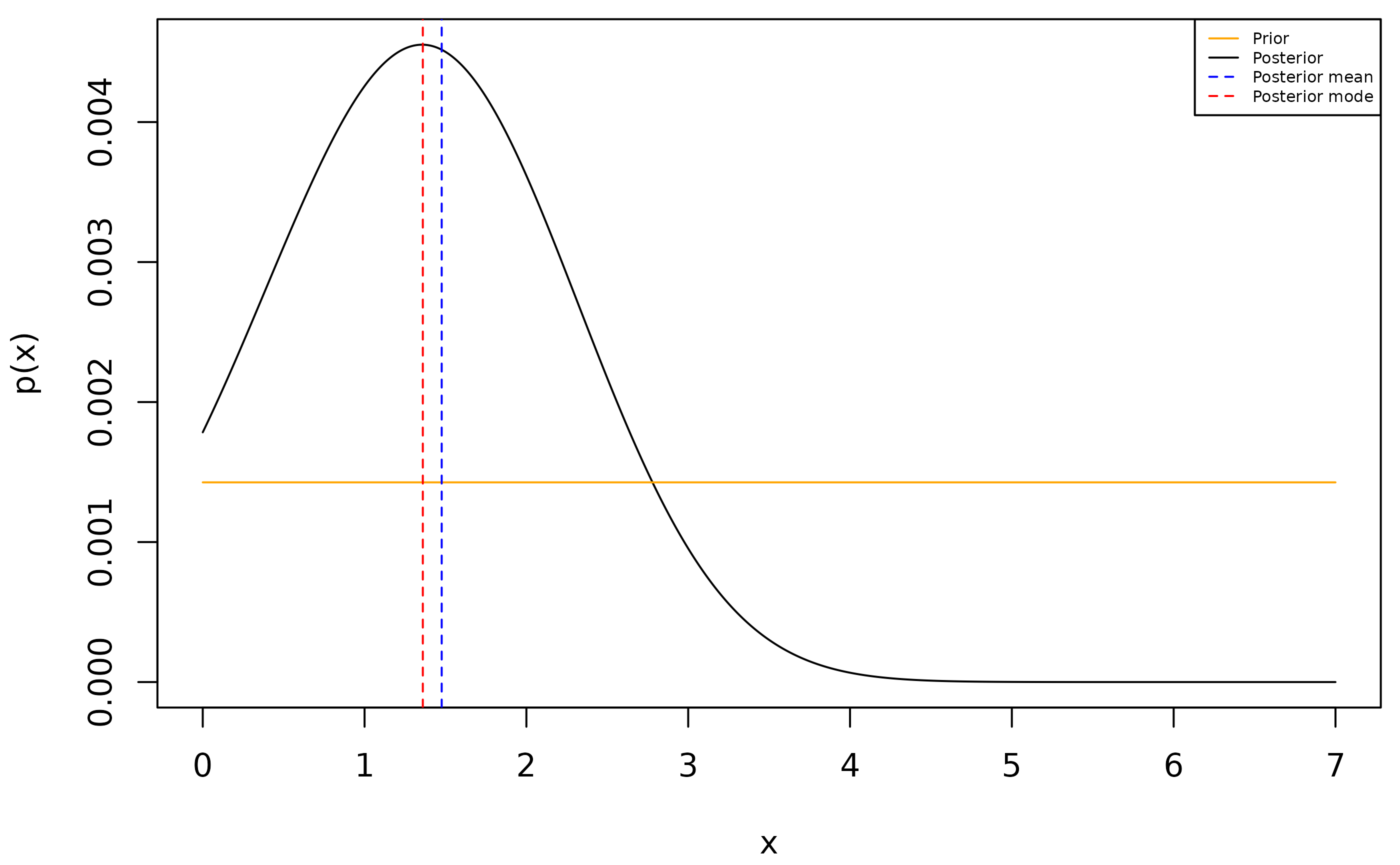
Another use of the posterior is to obtain an alternative estimate of R0. For instance, the following extracts the posterior mode rather than the mean:

post_mode <- posterior$supp[which.max(posterior$pmf)]
post_mode
#> [1] 1.36

Returning the posterior is suitable for visualization purposes. Below is a graph containing the uniform prior, final posterior distribution, posterior mean and posterior mode: